Tip

An interactive online version of this notebook is available, which can be accessed via

---

Alternatively, you may download this notebook and run it offline.

Compare lithium-ion battery models

We compare three one-dimensional lithium-ion battery models: the Doyle-Fuller-Newman (DFN) model, the single particle model (SPM), and the single particle model with electrolyte (SPMe). Further details on these models can be found in [4].

Key steps:

Comparing models consists of 6 easy steps:

1. Load models and geometry

2. Process parameters

3. Mesh the geometry

4. Discretise models

5. Solve models

6. Plot results

But, as always we first import pybamm and other required modules

%pip install "pybamm[plot,cite]" -q    # install PyBaMM if it is not installed
import os

import pybamm

os.chdir(pybamm.__path__[0] + "/..")

import matplotlib.pyplot as plt
import numpy as np

Note: you may need to restart the kernel to use updated packages.

1. Load models

Since the three models we want to compare are already implemented in PyBaMM, they can be easy loaded using:

dfn = pybamm.lithium_ion.DFN()
spme = pybamm.lithium_ion.SPMe()
spm = pybamm.lithium_ion.SPM()

To allow us to perform the same operations on each model easily, we create a dictionary of these three models:

models = {"DFN": dfn, "SPM": spm, "SPMe": spme}

Each model can then be accessed using:

models["DFN"]

<pybamm.models.full_battery_models.lithium_ion.dfn.DFN at 0x1208c3380>

For each model, we must also provide a cell geometry. The geometry is different for different models; for example, the SPM has solves for a single particle in each electrode whereas the DFN solves for many particles. For simplicity, we use the default geometry associated with each model but note that this can be easily changed.

geometry = {
    "DFN": dfn.default_geometry,
    "SPM": spm.default_geometry,
    "SPMe": spme.default_geometry,
}

2. Process parameters

For simplicity, we use the default parameters values associated with the DFN model, but change the current function to be an input so that we can quickly solve the model with different currents

param = dfn.default_parameter_values
param["Current function [A]"] = "[input]"

It is simple to change this to a different parameter set if desired.

We then process the parameters in each of the models and geometries using this parameter set:

for model_name, model in models.items():
    param.process_model(model)
    param.process_geometry(geometry[model_name])

3. Mesh geometry

We use the defaults mesh properties (the types of meshes and number of points to be used) for simplicity to generate a mesh of each model geometry. We store these meshes in a dictionary of similar structure to the geometry and models dictionaries:

mesh = {}
for model_name, model in models.items():
    mesh[model_name] = pybamm.Mesh(
        geometry[model_name], model.default_submesh_types, model.default_var_pts
    )

4. Discretise model

We now discretise each model using its associated mesh and the default spatial method associated with the model:

for model_name, model in models.items():
    disc = pybamm.Discretisation(mesh[model_name], model.default_spatial_methods)
    disc.process_model(model)

5. Solve model

We now solve each model using the default solver associated with each model:

timer = pybamm.Timer()
solutions = {}
t_eval = [0, 3600]  # time in seconds
for model_name, model in models.items():
    solver = pybamm.IDAKLUSolver()
    timer.reset()
    solution = solver.solve(model, t_eval, inputs={"Current function [A]": 1})
    print(f"Solved the {model.name} in {timer.time()}")
    solutions[model_name] = solution

Solved the Doyle-Fuller-Newman model in 68.203 ms
Solved the Single Particle Model in 15.638 ms
Solved the Single Particle Model with electrolyte in 32.645 ms

6. Plot results

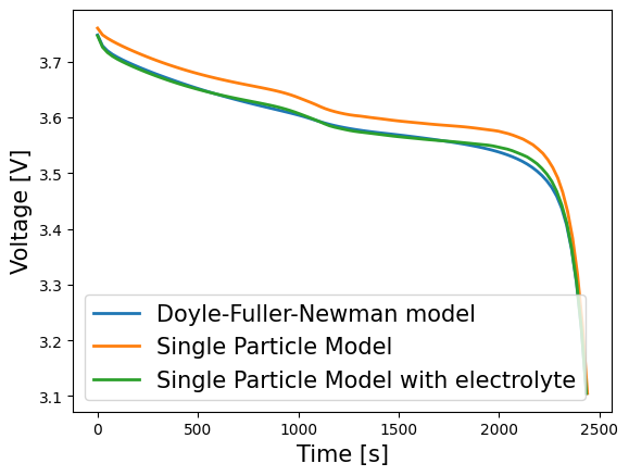
To plot results, we extract the variables from the solutions dictionary. Matplotlib can then be used to plot the voltage predictions of each models as follows:

for model_name, model in models.items():
    time_solution = solutions[model_name]["Time [s]"].entries
    time = np.linspace(time_solution[0], time_solution[-1], 100)
    voltage = solutions[model_name]["Voltage [V]"](time)
    plt.plot(time, voltage, lw=2, label=model.name)
plt.xlabel("Time [s]", fontsize=15)
plt.ylabel("Voltage [V]", fontsize=15)
plt.legend(fontsize=15)
plt.show()

Alternatively the inbuilt QuickPlot functionality can be employed to compare a set of variables over the discharge. We must first create a list of the solutions

list_of_solutions = list(solutions.values())

And then employ QuickPlot:

quick_plot = pybamm.QuickPlot(list_of_solutions)
quick_plot.dynamic_plot();

Changing parameters

Since we have made current an input, it is easy to change it and then perform the calculations again:

# update parameter values and solve again
# simulate for shorter time
t_eval = [0, 800]
for model_name, model in models.items():
    solutions[model_name] = model.default_solver.solve(
        model, t_eval, inputs={"Current function [A]": 3}
    )

# Plot
list_of_solutions = list(solutions.values())
quick_plot = pybamm.QuickPlot(list_of_solutions)
quick_plot.dynamic_plot();

By increasing the current we observe less agreement between the models, as expected.

References

The relevant papers for this notebook are:

pybamm.print_citations()

[1] Joel A. E. Andersson, Joris Gillis, Greg Horn, James B. Rawlings, and Moritz Diehl. CasADi – A software framework for nonlinear optimization and optimal control. Mathematical Programming Computation, 11(1):1–36, 2019. doi:10.1007/s12532-018-0139-4.
[2] Von DAG Bruggeman. Berechnung verschiedener physikalischer konstanten von heterogenen substanzen. i. dielektrizitätskonstanten und leitfähigkeiten der mischkörper aus isotropen substanzen. Annalen der physik, 416(7):636–664, 1935.
[3] Marc Doyle, Thomas F. Fuller, and John Newman. Modeling of galvanostatic charge and discharge of the lithium/polymer/insertion cell. Journal of the Electrochemical society, 140(6):1526–1533, 1993. doi:10.1149/1.2221597.
[4] Charles R. Harris, K. Jarrod Millman, Stéfan J. van der Walt, Ralf Gommers, Pauli Virtanen, David Cournapeau, Eric Wieser, Julian Taylor, Sebastian Berg, Nathaniel J. Smith, and others. Array programming with NumPy. Nature, 585(7825):357–362, 2020. doi:10.1038/s41586-020-2649-2.
[5] Alan C. Hindmarsh. The PVODE and IDA algorithms. Technical Report, Lawrence Livermore National Lab., CA (US), 2000. doi:10.2172/802599.
[6] Alan C. Hindmarsh, Peter N. Brown, Keith E. Grant, Steven L. Lee, Radu Serban, Dan E. Shumaker, and Carol S. Woodward. SUNDIALS: Suite of nonlinear and differential/algebraic equation solvers. ACM Transactions on Mathematical Software (TOMS), 31(3):363–396, 2005. doi:10.1145/1089014.1089020.
[7] Scott G. Marquis, Valentin Sulzer, Robert Timms, Colin P. Please, and S. Jon Chapman. An asymptotic derivation of a single particle model with electrolyte. Journal of The Electrochemical Society, 166(15):A3693–A3706, 2019. doi:10.1149/2.0341915jes.
[8] Valentin Sulzer, Scott G. Marquis, Robert Timms, Martin Robinson, and S. Jon Chapman. Python Battery Mathematical Modelling (PyBaMM). Journal of Open Research Software, 9(1):14, 2021. doi:10.5334/jors.309.