

Tip
An interactive online version of this notebook is available, which can be
accessed via

Alternatively, you may download this notebook and run it offline.
The PyBaMM Solvers#
PyBaMM has a few different solvers that can be used to solve the model equations. In this notebook we will go through the different solvers and contrast their features and performance.
[1]:
%pip install "pybamm[plot,cite]" -q    # install PyBaMM if it is not installed
import time

import matplotlib.pyplot as plt
import numpy as np

import pybamm
Note: you may need to restart the kernel to use updated packages.
The recommended solver in PyBaMM is the `pybamm.IDAKLUSolver <https://docs.pybamm.org/en/stable/source/api/solvers/idaklu_solver.html>`__: a direct wrapper around the Sundials IDAS solver, written and customised by the PyBaMM team to work well with PyBaMM’s models. It is the default solver for all models and is recommended for essentially all use cases.
Two experimental JAX-based solvers are also available:
`pybamm.IDAKLUJax<https://docs.pybamm.org/en/stable/source/api/solvers/idaklu_jax.html>`__ (experimental): a JAX wrapper around theIDAKLUSolverthat allows it to be used within a JAX model. Recommended for use on Linux or macOS.`pybamm.JaxSolver<https://docs.pybamm.org/en/stable/source/api/solvers/jax_solver.html>`__ (experimental): a pure JAX solver that uses thejaxlibrary to solve the model equations. Recommended for use on Linux or macOS.
Solver features#
Speed: The IDAKLU solver is fast both for solving models and for post-processing output variables.
Sensitivity analysis: The IDAKLU solver can compute forward model sensitivities with respect to input parameters, using the Sundials IDAS solver.
Adjoint sensitivity analysis: Either adjoint sensitivity analysis or reverse-mode auto differentiation is useful to compute sensitivities when the number of input parameters is very large (e.g. ML models). Currently only the pure JAX solver supports reverse-mode auto differentiation; adding adjoint sensitivity analysis to the IDAKLU solver is a future development goal.
Parallelism: If a list of input parameters is passed to the solver, the IDAKLU solver can solve the model in parallel for each parameter using multiple threads via OpenMP (useful, e.g., for parameter sweeps). If enough threads are available and the model is large enough, it can also parallelise a single solve using OpenMP and the Sundials NVECTOR_OPENMP implementation.
GPU acceleration: Currently only the pure JAX solver supports GPU acceleration. There is some experimental support for GPU acceleration via a new JAX-based backend for the IDAKLU solver, but this is still in development.
Events: The IDAKLU solver supports events, which trigger an action when a certain condition is met (the main use case being to stop the solver between steps of an experiment). It uses the underlying Sundials event handling, which is fast and robust. The pure JAX solver does not support events.
Evaluation and interpolation points: All solvers take a list of time points to evaluate the solution (the
t_evalargument), which stops the solver at each requested point. The IDAKLU solver can additionally take a list of interpolation points (thet_interpargument), interpolating the solution at these points without stopping the solver, speeding up the calculation.Other features: The Sundials solvers have many features that change how the solver works (tolerances, linear solvers, minimum step sizes, etc.); see the Sundials docs. Many of these are exposed and documented in the IDAKLU solver (see the docs). If PyBaMM does not expose a feature you need, please post an issue on the GitHub page.
Solver timing#
Below we look at the solve time for the IDAKLUSolver on the SPM, SPMe and DFN models with their default options, separating the first solve (which includes solver setup) from subsequent solves.
[2]:
first_solve_time = np.zeros(3)
second_solve_time = np.zeros(3)
model_classes = [
    pybamm.lithium_ion.SPM,
    pybamm.lithium_ion.SPMe,
    pybamm.lithium_ion.DFN,
]
for i, model_cls in enumerate(model_classes):
    sim = pybamm.Simulation(model_cls(), solver=pybamm.IDAKLUSolver())
    start_time = time.perf_counter()
    sol = sim.solve([0, 3600])
    voltage = sol["Voltage [V]"](0)
    first_solve_time[i] = time.perf_counter() - start_time
    start_time = time.perf_counter()
    sol = sim.solve([0, 3600])
    voltage = sol["Voltage [V]"](0)
    second_solve_time[i] = time.perf_counter() - start_time

labels = [m.__name__ for m in model_classes]
x = np.arange(3)
width = 0.35
fig, ax = plt.subplots(figsize=(7, 5))
ax.bar(x - width / 2, first_solve_time, width, label="First solve (incl. setup)")
ax.bar(x + width / 2, second_solve_time, width, label="Second solve")
ax.set_xticks(x)
ax.set_xticklabels(labels)
ax.set_ylabel("Time (s)")
ax.set_title("IDAKLUSolver solve time")
ax.legend()
plt.tight_layout()
plt.show()
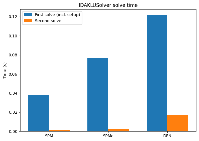
The “First solve” bars include the solver setup time, which for these relatively small problems is significant. The “Second solve” bars exclude this setup time and give a clearer indication of the solver’s speed for (a) calculating a solution and (b) post-processing the solution to extract the voltage.
The IDAKLU solver is customised to work well with PyBaMM’s models, and its online (via t_eval) and post-processing interpolation features mean obtaining output variables is fast.