

Tip
An interactive online version of this notebook is available, which can be
accessed via

Alternatively, you may download this notebook and run it offline.
Tutorial 4 - Setting parameter values#
In Tutorial 1 and Tutorial 2, we saw how to run a PyBaMM model with all the default settings. However, PyBaMM also allows you to tweak these settings for your application. In this tutorial, we will see how to change the parameters in PyBaMM.
[1]:
%pip install "pybamm[plot,cite]" -q    # install PyBaMM if it is not installed
import pybamm
Note: you may need to restart the kernel to use updated packages.
Change the whole parameter set#
PyBaMM has a number of in-built parameter sets (check the list here), which can be selected doing
[2]:
parameter_values = pybamm.ParameterValues("Chen2020")
The parameter values are stored in a dictionary-like object of class `pybamm.ParameterValues <https://docs.pybamm.org/en/latest/source/api/parameters/parameter_values.html>`__.
[3]:
parameter_values
[3]:
{'Ambient temperature [K]': 298.15,
 'Bulk solvent concentration [mol.m-3]': 2636.0,
 'Cation transference number': 0.2594,
 'Cell cooling surface area [m2]': 0.00531,
 'Cell thermal expansion coefficient [m.K-1]': 1.1e-06,
 'Cell volume [m3]': 2.42e-05,
 'Contact resistance [Ohm]': 0,
 'Current function [A]': 5.0,
 'EC diffusivity [m2.s-1]': 2e-18,
 'EC initial concentration in electrolyte [mol.m-3]': 4541.0,
 'Electrode height [m]': 0.065,
 'Electrode width [m]': 1.58,
 'Electrolyte conductivity [S.m-1]': <function electrolyte_conductivity_Nyman2008 at 0x1175f32e0>,
 'Electrolyte diffusivity [m2.s-1]': <function electrolyte_diffusivity_Nyman2008 at 0x1175f3240>,
 'Initial SEI thickness [m]': 5e-09,
 'Initial concentration in electrolyte [mol.m-3]': 1000.0,
 'Initial concentration in negative electrode [mol.m-3]': 29866.0,
 'Initial concentration in positive electrode [mol.m-3]': 17038.0,
 'Initial temperature [K]': 298.15,
 'Lithium interstitial reference concentration [mol.m-3]': 15.0,
 'Lower voltage cut-off [V]': 2.5,
 'Maximum concentration in negative electrode [mol.m-3]': 33133.0,
 'Maximum concentration in positive electrode [mol.m-3]': 63104.0,
 'Negative current collector conductivity [S.m-1]': 58411000.0,
 'Negative current collector density [kg.m-3]': 8960.0,
 'Negative current collector specific heat capacity [J.kg-1.K-1]': 385.0,
 'Negative current collector thermal conductivity [W.m-1.K-1]': 401.0,
 'Negative current collector thickness [m]': 1.2e-05,
 'Negative electrode Bruggeman coefficient (electrode)': 0,
 'Negative electrode Bruggeman coefficient (electrolyte)': 1.5,
 'Negative electrode OCP [V]': <function graphite_LGM50_ocp_Chen2020 at 0x106116340>,
 'Negative electrode OCP entropic change [V.K-1]': 0.0,
 'Negative electrode active material volume fraction': 0.75,
 'Negative electrode charge transfer coefficient': 0.5,
 'Negative electrode conductivity [S.m-1]': 215.0,
 'Negative electrode density [kg.m-3]': 1657.0,
 'Negative electrode double-layer capacity [F.m-2]': 0.2,
 'Negative electrode exchange-current density [A.m-2]': <function graphite_LGM50_electrolyte_exchange_current_density_Chen2020 at 0x1175f2ac0>,
 'Negative electrode porosity': 0.25,
 'Negative electrode reaction-driven LAM factor [m3.mol-1]': 0.0,
 'Negative electrode specific heat capacity [J.kg-1.K-1]': 700.0,
 'Negative electrode thermal conductivity [W.m-1.K-1]': 1.7,
 'Negative electrode thickness [m]': 8.52e-05,
 'Negative particle diffusivity [m2.s-1]': 3.3e-14,
 'Negative particle radius [m]': 5.86e-06,
 'Nominal cell capacity [A.h]': 5.0,
 'Number of cells connected in series to make a battery': 1.0,
 'Number of electrodes connected in parallel to make a cell': 1.0,
 'Open-circuit voltage at 0% SOC [V]': 2.5,
 'Open-circuit voltage at 100% SOC [V]': 4.2,
 'Positive current collector conductivity [S.m-1]': 36914000.0,
 'Positive current collector density [kg.m-3]': 2700.0,
 'Positive current collector specific heat capacity [J.kg-1.K-1]': 897.0,
 'Positive current collector thermal conductivity [W.m-1.K-1]': 237.0,
 'Positive current collector thickness [m]': 1.6e-05,
 'Positive electrode Bruggeman coefficient (electrode)': 0,
 'Positive electrode Bruggeman coefficient (electrolyte)': 1.5,
 'Positive electrode OCP [V]': <function nmc_LGM50_ocp_Chen2020 at 0x1175f2b60>,
 'Positive electrode OCP entropic change [V.K-1]': 0.0,
 'Positive electrode active material volume fraction': 0.665,
 'Positive electrode charge transfer coefficient': 0.5,
 'Positive electrode conductivity [S.m-1]': 0.18,
 'Positive electrode density [kg.m-3]': 3262.0,
 'Positive electrode double-layer capacity [F.m-2]': 0.2,
 'Positive electrode exchange-current density [A.m-2]': <function nmc_LGM50_electrolyte_exchange_current_density_Chen2020 at 0x1175f31a0>,
 'Positive electrode porosity': 0.335,
 'Positive electrode reaction-driven LAM factor [m3.mol-1]': 0.0,
 'Positive electrode specific heat capacity [J.kg-1.K-1]': 700.0,
 'Positive electrode thermal conductivity [W.m-1.K-1]': 2.1,
 'Positive electrode thickness [m]': 7.56e-05,
 'Positive particle diffusivity [m2.s-1]': 4e-15,
 'Positive particle radius [m]': 5.22e-06,
 'Ratio of lithium moles to SEI moles': 2.0,
 'Reference temperature [K]': 298.15,
 'SEI electron conductivity [S.m-1]': 8.95e-14,
 'SEI growth activation energy [J.mol-1]': 0.0,
 'SEI kinetic rate constant [m.s-1]': 1e-12,
 'SEI lithium interstitial diffusivity [m2.s-1]': 1e-20,
 'SEI open-circuit potential [V]': 0.4,
 'SEI partial molar volume [m3.mol-1]': 9.585e-05,
 'SEI reaction exchange current density [A.m-2]': 1.5e-07,
 'SEI resistivity [Ohm.m]': 200000.0,
 'SEI solvent diffusivity [m2.s-1]': 2.5e-22,
 'Separator Bruggeman coefficient (electrolyte)': 1.5,
 'Separator density [kg.m-3]': 397.0,
 'Separator porosity': 0.47,
 'Separator specific heat capacity [J.kg-1.K-1]': 700.0,
 'Separator thermal conductivity [W.m-1.K-1]': 0.16,
 'Separator thickness [m]': 1.2e-05,
 'Thermodynamic factor': 1.0,
 'Total heat transfer coefficient [W.m-2.K-1]': 10.0,
 'Upper voltage cut-off [V]': 4.2,
 'citations': ['Chen2020']}
and the specific values can be accessed using standard dictionary syntax:
[4]:
parameter_values["Electrode height [m]"]
[4]:
0.065
We can also search parameter values with a given keyword using the search command:
[5]:
parameter_values.search("electrolyte")
Results for 'electrolyte': ['EC initial concentration in electrolyte [mol.m-3]', 'Negative electrode Bruggeman coefficient (electrolyte)', 'Positive electrode Bruggeman coefficient (electrolyte)', 'Separator Bruggeman coefficient (electrolyte)', 'Initial concentration in electrolyte [mol.m-3]', 'Electrolyte diffusivity [m2.s-1]', 'Electrolyte conductivity [S.m-1]']
EC initial concentration in electrolyte [mol.m-3] -> 4541.0
Negative electrode Bruggeman coefficient (electrolyte) -> 1.5
Positive electrode Bruggeman coefficient (electrolyte) -> 1.5
Separator Bruggeman coefficient (electrolyte) -> 1.5
Initial concentration in electrolyte [mol.m-3] -> 1000.0
Electrolyte diffusivity [m2.s-1] -> <function electrolyte_diffusivity_Nyman2008 at 0x1175f3240>
Electrolyte conductivity [S.m-1] -> <function electrolyte_conductivity_Nyman2008 at 0x1175f32e0>
To run a simulation with a given parameter set, we can proceed as usual but passing the parameters as the parameter_values keyword argument
[6]:
model = pybamm.lithium_ion.DFN()
sim = pybamm.Simulation(model, parameter_values=parameter_values)
sim.solve([0, 3600])
sim.plot()
[6]:
<pybamm.plotting.quick_plot.QuickPlot at 0x1200e4980>
Change individual parameters#
We often want to quickly change a small number of parameter values to investigate how the behaviour or the battery changes. In such cases, we can change parameter values directly in notebook or script we are working in as we demonstrate in this section.
Parameters can either have a constant value or be a function of a model variable. These dependencies are hardcoded into the PyBaMM models. In order to check what are the specific parameters that a model requires, and whether they must be constants or they can be functions, we can call the print_parameter_info method.
[7]:
model.print_parameter_info()
┌───────────────────────────────────────────────────────────┬─────────────────────────────────────────────────────────────────────────────────────────────────────────────────────────────────────────────────────────────────────────────────────────────────────────────┐
│ Parameter │ Type of parameter │
├───────────────────────────────────────────────────────────┼─────────────────────────────────────────────────────────────────────────────────────────────────────────────────────────────────────────────────────────────────────────────────────────────────────────────┤
│ Separator thickness [m] │ Parameter │
│ Lower voltage cut-off [V] │ Parameter │
│ Initial temperature [K] │ Parameter │
│ Number of cells connected in series to make a battery │ Parameter │
│ Positive electrode Bruggeman coefficient (electrode) │ Parameter │
│ Positive electrode thickness [m] │ Parameter │
│ Nominal cell capacity [A.h] │ Parameter │
│ Maximum concentration in positive electrode [mol.m-3] │ Parameter │
│ Electrode width [m] │ Parameter │
│ Negative electrode Bruggeman coefficient (electrolyte) │ Parameter │
│ Number of electrodes connected in parallel to make a cell │ Parameter │
│ Reference temperature [K] │ Parameter │
│ Upper voltage cut-off [V] │ Parameter │
│ Negative electrode Bruggeman coefficient (electrode) │ Parameter │
│ Initial concentration in electrolyte [mol.m-3] │ Parameter │
│ Separator Bruggeman coefficient (electrolyte) │ Parameter │
│ Maximum concentration in negative electrode [mol.m-3] │ Parameter │
│ Electrode height [m] │ Parameter │
│ Negative electrode thickness [m] │ Parameter │
│ Positive electrode Bruggeman coefficient (electrolyte) │ Parameter │
│ Negative electrode active material volume fraction │ FunctionParameter with inputs(s) 'Through-cell distance (x) [m]', 'Horizontal distance (y) [m]', 'Vertical distance (z) [m]' │
│ Cation transference number │ FunctionParameter with inputs(s) 'Electrolyte concentration [mol.m-3]', 'Temperature [K]' │
│ Positive electrode OCP [V] │ FunctionParameter with inputs(s) 'Positive particle stoichiometry' │
│ Electrolyte diffusivity [m2.s-1] │ FunctionParameter with inputs(s) 'Electrolyte concentration [mol.m-3]', 'Temperature [K]' │
│ Negative electrode OCP entropic change [V.K-1] │ FunctionParameter with inputs(s) 'Negative particle stoichiometry' │
│ Ambient temperature [K] │ FunctionParameter with inputs(s) 'Distance across electrode width [m]', 'Distance across electrode height [m]', 'Time [s]' │
│ Negative electrode exchange-current density [A.m-2] │ FunctionParameter with inputs(s) 'Electrolyte concentration [mol.m-3]', 'Negative particle surface concentration [mol.m-3]', 'Maximum negative particle surface concentration [mol.m-3]', 'Temperature [K]' │
│ Positive electrode OCP entropic change [V.K-1] │ FunctionParameter with inputs(s) 'Positive particle stoichiometry' │
│ Positive electrode active material volume fraction │ FunctionParameter with inputs(s) 'Through-cell distance (x) [m]', 'Horizontal distance (y) [m]', 'Vertical distance (z) [m]' │
│ Separator porosity │ FunctionParameter with inputs(s) 'Through-cell distance (x) [m]', 'Horizontal distance (y) [m]', 'Vertical distance (z) [m]' │
│ Positive particle diffusivity [m2.s-1] │ FunctionParameter with inputs(s) 'Positive particle stoichiometry', 'Temperature [K]' │
│ Negative electrode OCP [V] │ FunctionParameter with inputs(s) 'Negative particle stoichiometry' │
│ Positive electrode exchange-current density [A.m-2] │ FunctionParameter with inputs(s) 'Electrolyte concentration [mol.m-3]', 'Positive particle surface concentration [mol.m-3]', 'Maximum positive particle surface concentration [mol.m-3]', 'Temperature [K]' │
│ Positive electrode porosity │ FunctionParameter with inputs(s) 'Through-cell distance (x) [m]', 'Horizontal distance (y) [m]', 'Vertical distance (z) [m]' │
│ Thermodynamic factor │ FunctionParameter with inputs(s) 'Electrolyte concentration [mol.m-3]', 'Temperature [K]' │
│ Initial concentration in positive electrode [mol.m-3] │ FunctionParameter with inputs(s) 'Radial distance (r) [m]', 'Through-cell distance (x) [m]' │
│ Current function [A] │ FunctionParameter with inputs(s) 'Time [s]' │
│ Negative particle radius [m] │ FunctionParameter with inputs(s) 'Through-cell distance (x) [m]' │
│ Positive electrode conductivity [S.m-1] │ FunctionParameter with inputs(s) 'Positive electrode stoichiometry', 'Temperature [K]' │
│ Negative particle diffusivity [m2.s-1] │ FunctionParameter with inputs(s) 'Negative particle stoichiometry', 'Temperature [K]' │
│ Electrolyte conductivity [S.m-1] │ FunctionParameter with inputs(s) 'Electrolyte concentration [mol.m-3]', 'Temperature [K]' │
│ Positive particle radius [m] │ FunctionParameter with inputs(s) 'Through-cell distance (x) [m]' │
│ Negative electrode porosity │ FunctionParameter with inputs(s) 'Through-cell distance (x) [m]', 'Horizontal distance (y) [m]', 'Vertical distance (z) [m]' │
│ Initial concentration in negative electrode [mol.m-3] │ FunctionParameter with inputs(s) 'Radial distance (r) [m]', 'Through-cell distance (x) [m]' │
│ Negative electrode conductivity [S.m-1] │ FunctionParameter with inputs(s) 'Negative electrode stoichiometry', 'Temperature [K]' │
└───────────────────────────────────────────────────────────┴─────────────────────────────────────────────────────────────────────────────────────────────────────────────────────────────────────────────────────────────────────────────────────────────────────────────┘
The table shows all the parameters that need to be provided to the model (in this case DFN). For example, we see that we need to define (amongst others) the Negative electrode thickness [m], which is defined to be a Parameter. This means it can only have a constant value. In contrast, other parameters are defined to be a FunctionParameter, which means that they can depend on model variables. For example, the Current function [A] is a FunctionParameter that can depend on
Time [s].
Note that a FunctionParameter can always be defined to be a constant (i.e. like if it was a Parameter), but a Parameter cannot be defined to be a function. This is because these dependencies are hardcoded in the model definitions.
Constant parameters#
Let’s start with a simple example: change the Current function [A] to be 10 A. To do this, we can simply update the value in the dictionary:
[8]:
parameter_values["Current function [A]"] = 10
Note that, as we mentioned above, even though Current function [A] could depend on time, we can always define it to be a function.
Now we just need to run the simulation with the new parameter values
[9]:
sim = pybamm.Simulation(model, parameter_values=parameter_values)
sim.solve([0, 3600])
sim.plot()
[9]:
<pybamm.plotting.quick_plot.QuickPlot at 0x120047530>
and we observe in the plot that now the applied current is indeed 10 A. Note that we still passed the interval [0, 3600] to sim.solve(), but the simulation terminated early as the lower voltage cut-off was reached.
Function parameters#
Let’s now illustrate how to change the Current function [A] to be a given time-dependent function. In this case we will set the current to be sinusoidal. To do this, we need to define the relevant function and pass it as a parameter.
[10]:
import numpy as np


def my_current(t):
    return pybamm.sin(2 * np.pi * t / 60)


parameter_values["Current function [A]"] = my_current
Note that the my_current function takes an argument t, which is time. PyBaMM will assume that the arguments are defined exactly as in the print_parameter_info table above, so the actual name given to the arguments does not matter, but the order does. For example, for the Electrolyte conductivity [S.m-1], it will assume that the first argument is Electrolyte concentration [mol.m-3] and the second is Temperature [K].
We can now solve the model again. In this case, we will pass t_eval to be an array of the points we want to evaluate our solution to the solver (rather than the start and end points only) to make sure we have enough time points to resolve the sinusoidal function in our output.
[11]:
sim = pybamm.Simulation(model, parameter_values=parameter_values)
t_eval = [0, 121]
sim.solve(t_eval=t_eval)
sim.plot(["Current [A]", "Voltage [V]"])
[11]:
<pybamm.plotting.quick_plot.QuickPlot at 0x122289130>
Input parameters#
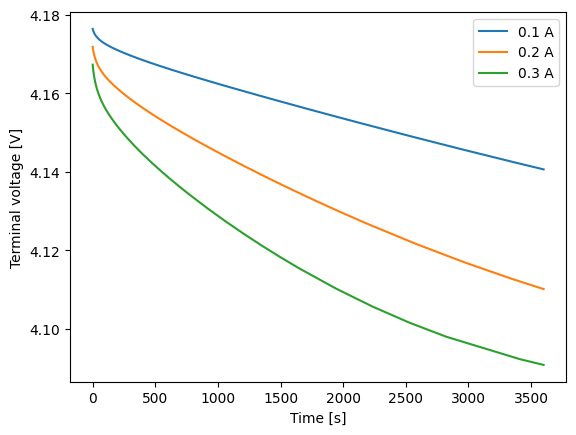
If the value of a parameter is expected to change often (e.g. running a parameter sweep) is is more convenient to set a parameter as an “input parameter”. This is a placeholder that can be filled in with a numerical value when the model is solved.
To set a parameter as an input parameter, we can set its value to the string [input] in the parameter values dictionary. For example, we can set the Current function [A] to be an input parameter and then run a parameter sweep over different current values like so:
[12]:
import matplotlib.pyplot as plt

parameter_values["Current function [A]"] = "[input]"
sim = pybamm.Simulation(model, parameter_values=parameter_values)
solns = []
for c in [0.1, 0.2, 0.3]:
    soln = sim.solve([0, 3600], inputs={"Current function [A]": c})
    plt.plot(soln["Time [s]"].entries, soln["Voltage [V]"].entries, label=f"{c} A")
    solns.append(soln["Terminal voltage [V]"].entries)
plt.xlabel("Time [s]")
plt.ylabel("Terminal voltage [V]")
plt.legend()
plt.show()
Define a new parameter set#
We can also define a new parameter set from scratch, which is useful if there is a new battery or chemistry on which we need to run simulations repeatedly. To do so, we can initialise a ParameterValues object and pass as an argument a dictionary of parameter values:
[13]:
def cube(t):
    return t**3


parameter_values = pybamm.ParameterValues(
    {
        "Negative electrode thickness [m]": 1e-4,
        "Positive electrode thickness [m]": 1.2e-4,
        "Current function [A]": cube,
    }
)
Note how, when we pass a function as a parameter, we pass the object without calling it, i.e. we pass cube rather than cube(t). This new parameter_values variable could now be passed to a simulation, but note that it is incomplete as it does not include all the parameters that the model needs to run (see the parameters needed by calling model.print_parameter_info(), as done above).
It is often convenient to define the parameter set in a separate file, and then call the parameters into your notebook or script. You can find some examples on how to do so in PyBaMM’s parameter library. You can copy one of the parameter sets available into a new file and modify it accordingly for the new parameter set. Then, whenever the set is needed, one can import the
get_parameter_values method from the corresponding file and call it to obtain a copy of the parameter values.
In this notebook we have seen how we can change the parameters of our model. In Tutorial 5 we show how can we define and run experiments.
References#
The relevant papers for this notebook are:
[14]:
pybamm.print_citations()
[1] Joel A. E. Andersson, Joris Gillis, Greg Horn, James B. Rawlings, and Moritz Diehl. CasADi – A software framework for nonlinear optimization and optimal control. Mathematical Programming Computation, 11(1):1–36, 2019. doi:10.1007/s12532-018-0139-4.
[2] Von DAG Bruggeman. Berechnung verschiedener physikalischer konstanten von heterogenen substanzen. i. dielektrizitätskonstanten und leitfähigkeiten der mischkörper aus isotropen substanzen. Annalen der physik, 416(7):636–664, 1935.
[3] Chang-Hui Chen, Ferran Brosa Planella, Kieran O'Regan, Dominika Gastol, W. Dhammika Widanage, and Emma Kendrick. Development of Experimental Techniques for Parameterization of Multi-scale Lithium-ion Battery Models. Journal of The Electrochemical Society, 167(8):080534, 2020. doi:10.1149/1945-7111/ab9050.
[4] Marc Doyle, Thomas F. Fuller, and John Newman. Modeling of galvanostatic charge and discharge of the lithium/polymer/insertion cell. Journal of the Electrochemical society, 140(6):1526–1533, 1993. doi:10.1149/1.2221597.
[5] Charles R. Harris, K. Jarrod Millman, Stéfan J. van der Walt, Ralf Gommers, Pauli Virtanen, David Cournapeau, Eric Wieser, Julian Taylor, Sebastian Berg, Nathaniel J. Smith, and others. Array programming with NumPy. Nature, 585(7825):357–362, 2020. doi:10.1038/s41586-020-2649-2.
[6] Alan C. Hindmarsh. The PVODE and IDA algorithms. Technical Report, Lawrence Livermore National Lab., CA (US), 2000. doi:10.2172/802599.
[7] Alan C. Hindmarsh, Peter N. Brown, Keith E. Grant, Steven L. Lee, Radu Serban, Dan E. Shumaker, and Carol S. Woodward. SUNDIALS: Suite of nonlinear and differential/algebraic equation solvers. ACM Transactions on Mathematical Software (TOMS), 31(3):363–396, 2005. doi:10.1145/1089014.1089020.
[8] Valentin Sulzer, Scott G. Marquis, Robert Timms, Martin Robinson, and S. Jon Chapman. Python Battery Mathematical Modelling (PyBaMM). Journal of Open Research Software, 9(1):14, 2021. doi:10.5334/jors.309.